Implementing a Generic A/B Testing Service

The ability to do A/B testing has become a key requirement of many tech driven companies. Without the ability to run meaningful A/B tests, how can we know for sure that changes and new features are resulting in the improvements that we anticipate? Here are a few examples of how A/B testing is used:

  • A social network, changing the number of required fields on their registration webpage and monitoring how it affects the percentage of visitors who register
  • An e-retailer, making a change to the way products are ordered by an e-commerce search engine and monitoring how it affects the number of product orders attributed to search
  • An advertiser, comparing statistical models used in placing advertisements and seeing which model leads to the highest click-through rate

In fact, any product which involves user interaction can be A/B tested to ensure that changes or new features are having a positive effect on relevant key performance indicators (KPIs).

In this post, I will discuss the motivation and benefits of implementing A/B testing as a generic service, to be shared and used throughout an organisation.

Consider the most simplistic implementation of A/B testing.
This will typically involve splitting the users of an application into two equal halves and then giving each of the two user groups a different experience. This could be achieved by adding some simple logic inside your application:

Here, we take the integer hash code of a user’s ID and apply modulo 2. Then, if we get an even number, give the user experience A and if we get an odd number, give the user experience B. We can store or log the experience given to each user and later compute some KPIs for the ‘odd’ users and the ‘even’ users and compare the two user groups.

This implementation should work fine, but in practice, there are a number of other things that are usually required from an A/B testing framework:

  1. Be able to disable a live experiment, or change the traffic allocation.
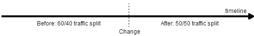
    For example, you might want to give just 1% of users a new feature and verify that it’s working as expected before ramping the traffic allocation up to a 50/50 test. In our simple implementation, the traffic allocation is hard-coded into the application, so we’d have to redeploy every time we make a change. Of course, we could use a database to store experiment configuration and make it possible to change the configuration while the application is running, but this is a lot more work to implement and requires you to maintain a database.

    Another concern here is around how you later perform your KPI analysis. Imagine a traffic allocation change being made to a live A/B test, at a certain point in time:

    Scenario where a traffic allocation change is made to a live A/B test.
    Scenario where a traffic allocation change is made to a live A/B test.

    When you perform KPI analysis to compare your experiments, it’s acceptable to perform the analysis before the change was made, or after the change was made, but not across the time of the change. This generally applies to any type of change – changes will affect your KPIs in some way and your results will not be meaningful if you analyse your experiments across the time when a change was made. It would be good if our A/B testing logic had some way of enforcing meaningful analysis.

  2. Have experiments with multiple parameters.
    In example above, there is just one parameter: a boolean indicating whether the new feature should be turned on or off. But it’s possible that you might want to have an experiment with many parameters, and these parameters may have different types. Hard-coding these parameters into your application will quickly become messy and hard to organise.

  3. Have multiple experiments running at the same time.
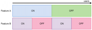
    Things can get tricky when you want to run multiple experiments at the same time. When is it OK for a user to be in two experiments at once? Of course, if you have several experiments testing the same thing (such as in the advertiser use case mentioned earlier, where there are several statistical models and you want to find which one yields the highest click-through rate), then a user can only be in one of those experiments. On the other hand, if you have two unrelated experiments which are testing completely independent features, then it’s fine for a user to be in both experiments at the same time.

    There are further complexities around how to allocate traffic fairly when users are being assigned to multiple experiments. Consider the case where we are A/B testing two new, independent features. For each feature, we want to find out whether it’s better to have that feature enabled or disabled. The scenario is depicted in the below image:

    A/B testing two independent experiments simultaneously, with an unfair traffic allocation scheme.
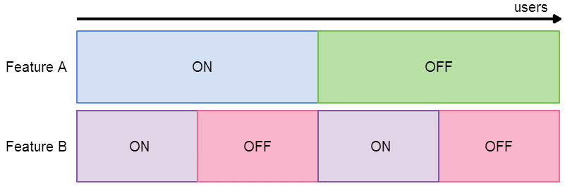
    A/B testing two independent experiments simultaneously, with an unfair traffic allocation scheme.

    Here, if you imagine that users are distributed horizontally across the diagram, then drawing a vertical line anywhere on the diagram would represent a single user’s experience. Here, if a user is assigned the experiment Feature A: On, they will also be assigned Feature B: On. So, if we later analyse the KPIs for the purple users vs the red users, we will have no idea whether any change in the KPIs has come from Feature A or Feature B. We need to allocate traffic in a fair way:

    A/B testing two independent experiments simultaneously, with a fair traffic allocation scheme.
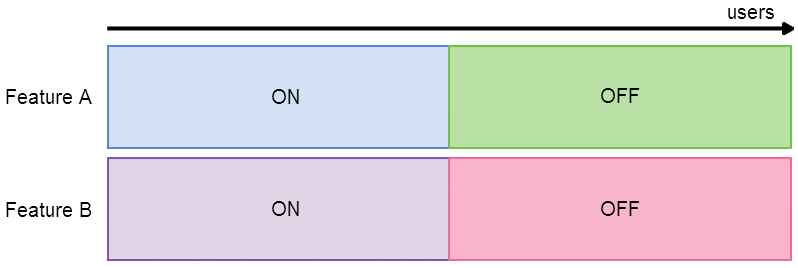
    A/B testing two independent experiments simultaneously, with a fair traffic allocation scheme.

    Here, the users assigned Feature A: On are equally split over Feature B: On and Feature B: Off. Now, if we look at the KPIs for the purple users vs the red users, we know that any change we see is purely down to Feature B.

    In this example, the solution is quite obvious, but what if we are testing many more features simultaneously – some of which have more than two variations. We need a way to ensure traffic is always allocated fairly, in any situation.

  4. Introduce segmentation logic.
    This is where you want your experiments to behave differently depending on the situation. For example, you might want an experiment to only be applicable to users from a certain country. Again, if you are writing your own A/B testing logic, this is more work for you to implement in your application.

  5. Validate experiments before they go live.
    In particular, this applies in the case where your experiments have many parameters of different types. There’s always the possibility of human error when you are configuring or making changes to an experiment. It would be nice to have a way to validate experiment configuration and ensure we are setting the right parameters with the correct types.

Implementing all of these features is a lot of work – and certainly not something you want to repeat in every application you develop that has some form of A/B testing requirement. A nice solution is to build an A/B testing service which handles things like storing experiment configuration, validation, segmentation, running multiple experiments simultaneously and allocating traffic fairly. Such a service could be used in two ways:

  1. By people: to define, configure and manage experiments
  2. By an application: to retrieve a set of parameters for handling a specific request

This can be hugely beneficial for anyone building an application that wants to do A/B testing. Instead of implementing a load of A/B testing logic in your application, your application just needs to make a single call to a service – effectively asking the question ‘what experience should I give this user?’. With this design, a client application just needs to pass a userId (or some other data element to use to split traffic into experiments) and a set of attributes which may be used for segmentation (for example, country=denmark might be an attribute). The client will then receive a response with a set of parameters which it can use to determine what experience to give the user. Using our earlier example, the response parameters would consist of something like featureEnabled=true. No other A/B testing logic needs to be implemented in the application itself!

Having a generic A/B testing service clearly brings many benefits when you have multiple applications that need this type of functionality. But, there is a notable drawback to the scheme described above which I came across when building an A/B testing service to be used in my organisation. This design assumes that it is feasible to make a request to a separate service for every request processed by the application. There are two potential issues with this assumption: the first being that in super-low latency applications, adding a couple of milliseconds to the response time may be unacceptable, and the second being that in high-load applications, the volume of requests may be too high for it to be feasible to call an external service on every request.

We hit the second issue – as we have an application which handles hundreds of thousands of requests per second and it wasn’t feasible to give the A/B testing service enough resource to handle that kind of volume. Our solution was to allow this application to download experiment traffic allocation instructions periodically from our service and implement some additional A/B testing logic in the application. This solution is not as clean as the call-on-every-request approach as it requires more work in the client application, such as segmentation logic, but the application still benefits from the service handling configuration storage, validation and traffic allocation.

For a more detailed description of the logic behind handling multiple simultaneous experiments, check out my next post (originally published on the Adform engineering blog). I also recommend reading this paper from Google, which the ideas in this post are based on.

Building a Search Engine for E-Commerce with Elasticsearch

This is a continuation of my previous post on search engines. Having been involved with using Elasticsearch to build a search engine for e-commerce, there are some interesting ideas which I have taken away from the experience. I will go through some of the design decisions made and problems encountered along the way.

Tweaking the Search Query
Elasticsearch provides a huge variety of different query types, each of which has a different approach to retrieving search results. For example, the term query will find documents containing a certain term, the fuzzy query will match documents containing terms which are approximately equal to a given term, the geo-shape query enables you to perform useful queries over documents containing longitude and latitude coordinates and many more. Any of these query types can be composed using compositional query types, such as the bool query.

When I talk about tweaking the search query, I mean choosing the query types to use and structuring our query in a way that will enable us to achieve optimal results for any kind of search over the product base. The two main properties of the search query which we are trying to optimise are:

  1. How to best determine which products match
  2. How to best determine the order (i.e. relative importance) of the matching products

One of the first options that we considered using was the query-string query: a query type that parses your query and decides what query types to use, and often does the sensible thing. For instance, jeans will match any document containing the term jeans, blue jeans will match any document containing both ‘blue’ and ‘jeans’ and "blue jeans" will match documents containing both terms together (an exact match). You can even make more complex searches, like blue jeans -(levi OR diesel) which will match documents containing ‘blue’ and ‘jeans’ but not the terms ‘levi’ or ‘diesel’. This all seems quite nice at first, but this query type can give very unexpected results if used incorrectly – for example t-shirt will match documents containing ‘t’, but will exclude all documents containing ‘shirt’. Of course, customers can’t be expected to understand why this happens or how to fix their query.

Another option is the multi-match query, which takes a list of fields to query over and builds a sequence of match queries. Similar to the query-string query, each field can each be given a different boost factor, which is used in determining relative importance of some terms matching a given field. You can also tweak the type of multi_match – e.g. whether the query terms must all be found in a single field, or can be found in different fields (but not necessarily in the same field). Here is an example of a multi_match query:

{
  "multi_match" : {
    "query":      "gladiator russell crowe",
    "type":       "best_fields",
    "fields":     [ "title^10", "actors^5", "description^1" ]
  }
}

Here, we have used the boost operator (^) to indicate that the title field should be given the most importance. The query will still be matched against the description field, but matches in the title and actors fields will be given a higher score and will appear first in our result set. The best_fields type gives precedence when the query terms appear in the same field, but they don’t have to.

When matching across multiple fields, it can be tricky to figure out which documents are most relevant to the query. If we just consider which fields matched the query, then we won’t get optimal results. For example, if the query is ps4 controller and a document contains ‘ps4’ in the title field and ‘controller’ in the description field, then should it be given a higher score than a document which contains both terms in the title field but neither in the description field? The first document has more matching fields, but intuitively, the second document should surely be considered a more relevant result. Elasticsearch provides a solution to this: the disjunction-max (dis-max) query. This enables us to perform sub-queries over multiple fields and take the score of the best matching field (i.e. the maximum scoring sub-query), instead of summing the scores from each matching sub-query. In practice, this often yields better results and is in fact the default behaviour for the multi-match query.

We used the multi-match query successfully in production for quite some time, but ultimately decided to switch to using the common terms query. This is an interesting query type which provides not only a way to determine stop words dynamically, but also a way to not completely disregard stop words at search time. When using the multi-match query, we assigned a stop word filter to each field in our mapping, which uses a pre-defined list of stop words to remove the most common and semantically useless words from the index. This is usually good because those words don’t add much meaning and make searching the index slower. But is this always a good thing? Consider the video game ‘The Last Of Us’. A search for the last of us would result in all products containing the term ‘last’ and those products would not be ordered very sensibly, since the other three terms (all stop words) would have been thrown away. In this scenario, the common terms query is much more effective. Instead of removing stop words, it uses term frequencies across the whole index to determine which terms are important and which occur frequently enough to be considered stop words. In this example, ‘last’ would likely be deemed an important term, while ‘the’, ‘of’ and ‘us’ would be deemed less important. The common terms query then splits searching into two steps:

  1. Use the important terms to determine the result set
  2. Use the less important terms to order the result set

This way, stop words are not completely thrown away, but they are not considered until after the product result set has been determined. This fits very nicely with the two search query properties we are trying to optimise towards. To keep the cross-field search benefits of the multi-match, the common terms query can be wrapped inside a dis-max and have a boost factor applied to each field:

{
  "dis_max" : {
    "tie_breaker" : 0.3,
    "queries" : [
      {
       "common": {
          "title": {
          "query": "the last of us",
          "boost": 10,
          "cutoff_frequency": 0.001
          }
       }
      },
      {
        "common": {
          "studio": {
          "query": "the last of us",
          "boost": 3,
          "cutoff_frequency": 0.001
          }
        }
      },
      {
        "common": {
          "description": {
          "query": "the last of us",
          "boost": 1,
          "cutoff_frequency": 0.001
          }
        }
      }
    ]
  }
}

With this query, we saw an uplift in product page visits from search and more customers were clicking products returned in the first two rows of their search results. This demonstrates that our use of the common terms query was enabling customers to find the most relevant products more easily.

Customising the Score Function
As we’ve seen, Elasticsearch provides us with many clever ways to score search results such that the most relevant products appear first. But in e-commerce, there are some factors that are worth considering outside of how relevant the product itself is. This includes things like:

  • How popular is the product?
  • Is the product in stock?
  • Was the product released recently?
  • How profitable are sales of the product?

For example, if a product is extremely popular at the moment, then perhaps it should be boosted above other search results. Or, if a product is out of stock, we probably don’t want to show it in the first few search results.

To factor in this information, we can design our own scoring function which will adjust the scores computed by our Elasticsearch query. This is done by wrapping the main search query in a custom_score query. We can then provide a script which modifies the original score (denoted by _score) by using fields from the index and a set of parameters. This way, we could index a field such as ‘product_popularity’ into our product documents, and then boost the _score for more popular products. We would make it possible to assign different levels of importance to each factor with an adjustable weighting for each parameter. Normalisation is also important to ensure we operate on the same scale for each factor. Here’s an example of this with just the product popularity factor:

"custom_score": {
    "params": {
        "scoreWeighting": 2,
        "popularityWeighting": 5,
        "maxPopularity": x
    },
    "query": {...},
    "script": "scoreWeighting * _score + (popularityWeighting * (doc['popularity'].value / maxPopularity))"
}

In practice, our score function considers a lot more than the product popularity and is dynamically generated by the search service using a set of configurable parameters which can be changed at any time without a redeployment.

Achieving Faceted Search
Faceted search is a way of enhancing the search experience by enabling the user to navigate their search results by applying a set of filters. Faceted navigation is now seen on the majority of online retail sites and probably looks very familiar to you:

An example of faceted search

A facet is a set of filters. In the above example, there are three facets: category, sub-category and price. Sometimes, more complex faceting may be desirable – for instance, you might want it so when you apply the ‘DVD’ category filter, you are then given a choice of movie genres to filter by. This is called a nested facet, as it is a facet within a facet.

With Elasticsearch, it is fairly painless to set up faceted search. First, you will need to have in your mapping a non-analysed version of each field you want to facet on:

{
    "category": {
        "type":     "string",
        "index":    "not_analyzed"
    }
}

We use the not_analyzed setting because at index time we want the field to be mapped as an exact field, so that later, the filter options (in this case categories) will appear exactly as they were indexed.

Now, at query time, we can append a terms aggregation to our query:

{
    "aggs" : {
        "categories" : {
            "terms" : { "field" : "category" }
        }
    }
}

Our response will now contain all the information we need about categories for the given query. Elasticsearch will give us a breakdown of counts for each type of category within the result set for our query:

 "aggregations" : {
        "categories" : {
            "doc_count_error_upper_bound": 0, 
            "sum_other_doc_count": 0, 
            "buckets" : [ 
                {
                    "key" : "Merchandise",
                    "doc_count" : 856
                },
                {
                    "key" : "Clothing",
                    "doc_count" : 455
                },
                ... etc ...
            ]
        }
    }
}

Now, when a user clicks on a category, such as Clothing, we usually want our search results to be filtered to display only clothing, however the facet counts for categories should remain unchanged – the Merchandise facet count should still be 856. To achieve this, we can use Elasticsearch filters instead of extending the query. In this example, we would append a terms filter on the category field, with the term ‘Clothing’. This will achieve the behaviour we want because filters are not considered when computing the facet counts – the search results will be filtered, but the facet counts will remain unchanged.

Implementing Instant Search
Instant search is where the search engines assists you with your search while you type. There are several variants of this:

  1. Displaying products relevant to what the customer has typed so far
  2. Displaying search suggestions – predicting what the customer is going to type next (AKA auto-complete)
  3. Detecting spelling mistakes and suggesting corrections

It is actually possible to achieve all of the above with a single Elasticsearch query! We achieved this by using an n-grams analyzer for auto-complete, a shingle analyzer for search suggestions and Elasticsearch’s in-built term and phrase suggester for spelling correction. Check out my colleague’s post here for a complete example of how to achieve this.

Handling Distributed Search
Elasticsearch is an excellent example of a sophisticated distributed system which hides much of the inherent complexity from the user. Behind the scenes, problems like partitioning documents into shards, balancing shards across the cluster, replicating data to maintain fault-tolerance and efficiently routing requests between nodes are handled. All you have to do is configure a couple of settings in your elasticsearch.yaml – such as the number of shards to split each index into and the number of replicas to keep of each shard.

While configuring distributed search is pretty easy, there are some more complex issues which should be addressed. One of these issues is: how can we make a change to our mapping (i.e. the index) without causing any downtime to our search engine. For an e-commerce company, any form of downtime translates directly to a loss in revenue, and with our large product base, re-populating the search indices is a lengthy process which takes several hours. This problem can be solved using index aliases – an Elasticsearch feature which enables us to set up something similar to a symbolic link – an index alias which always points to a live and fully prepared index. For example, we can set up an alias, products which points to a specific version of our products index:

PUT /products_v1/_alias/products

Now, we can make a change to our mapping and populate a new index, products_v2, wait until we are satisfied that all data has been indexed and shards balanced, before finally switching our alias to point to the new index.

There are some problems that come with the distributed nature of Elasticsearch. Imagine performing a search, getting 10 search results in the response, then refreshing the page and seeing 50 search results. How can search be non-deterministic?! Well, this is a problem that we encountered. This problem comes about as a result of Elasticsearch making optimisations and using approximate term frequencies to determine results. Each shard has a subset of documents in the index, and by default, Elasticsearch will use the shard’s term frequencies as an approximation for the actual term frequencies. When using the common terms query as described earlier, a term may fall under the threshold for being considered a stop word on one shard, but may be over the threshold on another shard. So, depending on which node a query gets routed to, we can end up with different results. Most of the time, this isn’t a problem as term frequencies should be very similar across all shards, providing there is enough data and the data is evenly distributed. But, if it does become a problem, full accuracy can be achieved by changing the default query type to dfs_query_and_fetch, by appending &search_type=dfs_query_then_fetch to the search URI. This query type performs an additional round-trip, collecting term frequencies from all nodes and calculating a global term frequency, before sending the query to all shards and computing results using the global frequencies. This ensures results are always accurate, but comes at the cost of some additional latency.

A similar problem can be seen in faceting. Facet counts are computed on each shard and then aggregated on the node designated as coordinator. If, say, our request is for the top 10 terms within a facet, then each node will return it’s locally computed top 10 facet elements. In cases where there are more than 10 terms, accuracy can be lost. To address this problem, a recent version of Elasticsearch introduced a shard_size attributed which can be set on the facet query, and specifies the number of elements each shard should return. This is separate from the size attribute – i.e. the number of elements we actually want. Asking each shard to return more elements is of course more expensive, but will give higher accuracy when it is needed.

Conclusions

  • It is hard to find a query which works well for every search. If there is a particular search found to yield bad results, it can be easy to optimise towards improving and fixing that search, but then other searches end up suffering as a result. When making changes to the search query, always think: will this work well for both general searches and specific searches?
  • Use filters for faceting, to filter search results without affecting facet counts. Also, Elasticsearch filters are (by default) cached, so can boost performance.
  • The three types of instant search: product suggestions, search suggestions and spelling corrections can be achieved with a single Elasticsearch query – providing the title field is configured with both a shingles and n-grams analyzer.
  • You should always A/B test whenever you make a change to the search experience. It can be invaluable to have good reporting on things like ‘searches which yield no results’ to easily catch problem with changes to the query.
  • Use index aliases to make large changes while maintaining zero-downtime.
  • There can be non-deterministic results with a distributed search engine, but with Elasticsearch these problems can be resolved at the cost of additional latency.
  • The search experience makes a big difference. It not only enables customers to discover the products they are looking for, but a well-tuned search experience can also can help them discover things they weren’t explicitly searching for. We saw significant boosts in revenue from search every time we made improvements to the search engine.